Image Segmentation

• Non-contextual thresholding
  • Simple thresholding
  • Adaptive thresholding
  • Colour thresholding
• Contextual segmentation: Region growing
  • Pixel connectivity
  • Region similarity
  • Region growing
  • Split-and-merge segmentation
• Texture segmentation: Spectral features
• References

Segmentation partitions an image into distinct regions containing each pixels with similar attributes. To be meaningful and useful for image analysis and interpretation, the regions should strongly relate to depicted objects or features of interest. Meaningful segmentation is the first step from low-level image processing transforming a greyscale or colour image into one or more other images to high-level image description in terms of features, objects, and scenes. The success of image analysis depends on reliability of segmentation, but an accurate partitioning of an image is generally a very challenging problem.
Segmentation techniques are either contextual or non-contextual. The latter take no account of spatial relationships between features in an image and group pixels together on the basis of some global attribute, e.g. grey level or colour. Contextual techniques additionally exploit these relationships, e.g. group together pixels with similar grey levels and close spatial locations.

Non-contextual thresholding

Thresholding is the simplest non-contextual segmentation technique. With a single threshold, it transforms a greyscale or colour image into a binary image considered as a binary region map. The binary map contains two possibly disjoint regions, one of them containing pixels with input data values smaller than a threshold and another relating to the input values that are at or above the threshold. The former and latter regions are usually labelled with zero (0) and non-zero (1) labels, respectively. The segmentation depends on image property being thresholded and on how the threshold is chosen.
Generally, the non-contextual thresholding may involve two or more thresholds as well as produce more than two types of regions such that ranges of input image signals related to each region type are separated with thresholds. The question of thresholding is how to automatically determine the threshold value.

Simple thresholding

The most common image property to threshold is pixel grey level: g(x,y) = 0 if f(x,y) < T and g(x,y) = 1 if f(x,y) ≥ T, where T is the threshold. Using two thresholds, T₁ < T₁, a range of grey levels related to region 1 can be defined: g(x,y) = 0 if f(x,y) < T₁ OR f(x,y) > T₂ and g(x,y) = 1 if T₁ ≤ f(x,y) ≤ T₂.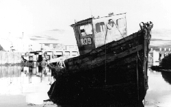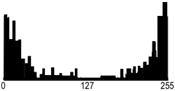

Greyscale image "Boat"	Its grey level histogram
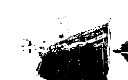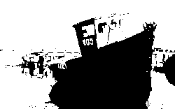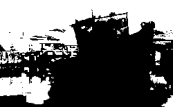Binary regions for T = 26	Binary regions for T = 133	Binary regions for T = 235
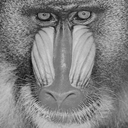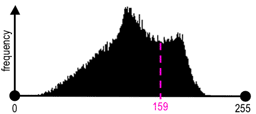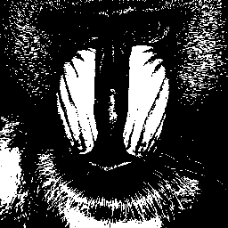Greyscale image "Baboon"	Its grey level histogram	Binary regions for T = 159

The main problems are whether it is possible and, if yes, how to choose an adequate threshold or a number of thresholds to separate one or more desired objects from their background. In many practical cases the simple thresholding is unable to segment objects of interest, as shown in the above images.
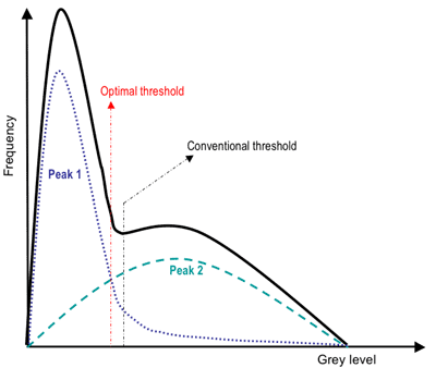
A general approach to thresholding is based on assumption that images are multimodal, that is, different objects of interest relate to distinct peaks (or modes) of the 1D signal histogram. The thresholds have to optimally separate these peaks in spite of typical overlaps between the signal ranges corresponding to individual peaks. A threshold in the valley between two overlapping peaks separates their main bodies but inevitably detects or rejects falsely some pixels with intermediate signals. The optimal threshold that minimises the expected numbers of false detections and rejections may not coincide with the lowest point in the valley between two overlapping peaks:

Adaptive thresholding

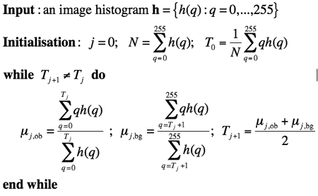
Since the threshold separates the background from the object, the adaptive separation may take account of empirical probability distributions of object (e.g. dark) and background (bright) pixels. Such a threshold has to equalise two kinds of expected errors: of assigning a background pixel to the object and of assigning an object pixel to the background. More complex adaptive thresholding techniques use a spatially varying threshold to compensate for local spatial context effects (such a spatially varying threshold can be thought as a background normalisation).
A simple iterative adaptation of the threshold is based on successive refinement of the estimated peak positions. It assumes that (i) each peak coincides with the mean grey level for all pixels that relate to that peak and (ii) the pixel probability decreases monotonically on the absolute difference between the pixel and peak values both for an object and background peak. The classification of the object and background pixels is done at each iteration j by using the threshold T_j found at previous iteration. Thus, at iteration j, each grey level f(x,y) is assigned first to the object or background class (region) if f(x,y) ≤ T_j or f(x,y) > T_j, respectively. Then, the new threshold, T_j+1 = 0.5(μ_j,ob + μ_j,bg) where μ_j,ob and μ_j,bg denote the mean grey level at iteration j for the found object and background pixels, respectively:

Colour thresholding

Color segmentation may be more accurate because of more information at the pixel level comparing to greyscale images. The standard Red-Green-Blue (RGB) colour representation has strongly interrelated colour components, and a number of other colour systems (e.g. HSI Hue-Saturation-Intensity) have been designed in order to exclude redundancy, determine actual object / background colours irrespectively of illumination, and obtain more more stable segmentation. An example below (from http://www.matrix-vision.com/products/software) shows that colour thresholding can focus on an object of interest much better than its greyscale analogue: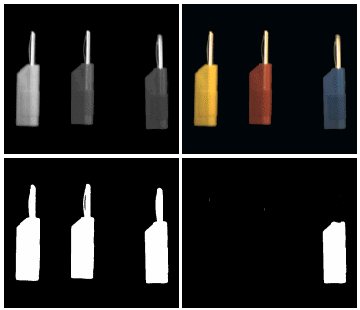

Greyscale vs. colour thresholding Segmentation of colour images involve a partitioning of the colour space, i.e. RGB or HSI space. One simple approach is based on some reference (or dominant) colour (R₀, G₀, B₀) and thresholding of Cartesian distances to it from every pixel colour f(x,y) = (R(x,y),G(x,y),B(x,y)):

where g(x,y) is the binary region map after thresholding. This thresholding rule defines a sphere in RGB space, centred on the reference colour. All pixels inside or on the sphere belong to the region indexed with 1 and all other pixels are in the region 0.
Also, there can be an ellipsoidal decision surface if independent distance thresholds are specified for the R, G, and B components. Generally, colour segmentation, just as the greyscale one, may be based on the analysis of 3D colour histograms or their more convenient 2D projections. A colour histogram is built by partitioning of the colour space onto a fixed number of bins such that the colours within each bin are considered as the same colour. An example below of the partitioned 11×11×11 RGB colour space is from (http://www.owlnet.rice.edu/~elec301/Projects02/artSpy/color.html):

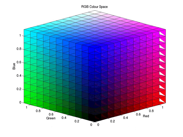
How fine should be the partitioning depends on the application domain. In many cases colour segmentation exploits only a few dominant colours corresponding to distinct peaks of the pixel-wise colour distribution (both the images and histograms below are from ij-plugins.sourceforge.net/ij-vtk/color-space/):

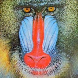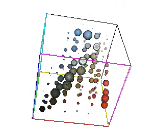Colour image "Baboon"	Its colour 6×6×6 histogram (sphere-size-coded bin values)
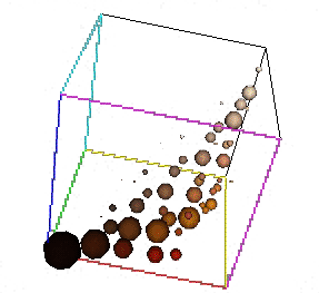Colour image "Clown"	Its colour 6×6×6 histogram (sphere-size-coded bin values)

If a chosen colour space separates colourless intensity values from intensity-independent colour components (such as hue and saturation or normalised red / blue colurs), colour segmentation can be based on a few pre-selected colours, e.g. on the eight primary colours (black, red, green, blue, yellow, cyan, magenta, white). An example below shows a digitised picture of the Rembrandt's canvas "Doctor Nicolaes Tulp's Demonstration of the Anatomy of the Arm" (1632; Mauritshuis Museum, The Hague, The Netherlands), its 8-bin histogram of the primary colours, and the corresponding colour regions:

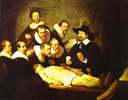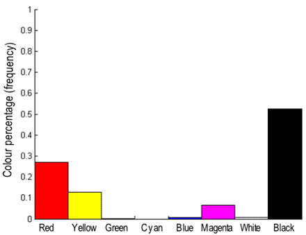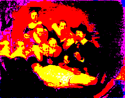Digitised Rembrandt's canvas	Colour 8-bin histogram	Regions of the primary colours
(www.abcgallery.com/R/rembrandt/)	(http://rsb.info.nih.gov/ij/plugins/color-inspector.html)

More efficient adaptive thresholding of greyscale images can be extended to colour images, too, by replacing mean grey levels for each colour region with its mean colors, e.g. RGB-vectors with the mean component values.

Contextual segmentation: Region growing

Non-contextual thresholding groups pixels with no account of their relative locations in the image plane. Contextual segmentation can be more successful in separating individual objects because it accounts for closeness of pixels that belong to an individual object. Two basic approaches to contextual segmentation are based on signal discontinuity or similarity. Discontinuity-based techniques attempt to find complete boundaries enclosing relatively uniform regions assuming abrupt signal changes across each boundary. Similarity-based techniques attempt to directly create these uniform regions by grouping together connected pixels that satisfy certain similarity criteria. Both the approaches mirror each other, in the sense that a complete boundary splits one region into two.

Pixel connectivity

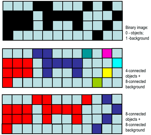
Pixel connectivity is defined in terms of pixel neighbourhoods. A normal rectangular sampling pattern producing a finite arithmetic lattice {(x,y): x = 0, 1, ..., X−1; y = 0, 1, ..., Y−1} supporting digital images allows us to define two types of neighbourhood surrounding a pixel. A 4-neighbourhood {(x−1,y), (x,y+1), (x+1,y), (x,y−1)} contains only the pixels above, below, to the left and to the right of the central pixel (x,y). An 8-neighbourhood adds to the 4-neighbourhood four diagonal neighbours: {(x−1,y−1),(x−1,y), (x−1,y+1), (x,y+1), (x+1,y+1), (x+1,y), (x+1,y−1), (x,y−1)}.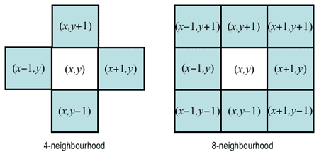
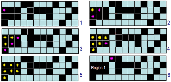
A 4-connected path from a pixel p₁ to another pixel p_n is defined as the sequence of pixels {p₁, p₂, ..., p_n} such that p_i+1 is a 4-neighbour of p_i for all i = 1, ..., n−1. The path is 8-connected if p_i+1 is an 8-neighbour of p_i. A set of pixels is a 4-connected region if there exists at least one 4-connected path between any pair of pixels from that set. The 8-connected region has at least one 8-connected path between any pair of pixels from that set.
One of the simplest and most common algorithms for labelling connected regions after greyscale or colour thresholding exploits the "grassfire" or "wave propagation" principle: after a "fire" or "wave" starts at one pixel, it propagates to any of the pixel's 4- or 8-neighbours detected by thresholding. Each already visited (i.e. "burnt away" or "wet") pixel cannot be visited again, and after the entire connected region is labelled, its pixels are assigned a region number, and the procedure continues to search for the next connected region. Magenta and yellow stars below indicate the fire, or wave front and the burnt away pixels, respectively. To label a region, the fire starts from its first chosen pixel:
The 4- and 8-connectivity produce different segmentation results:
Moreover, each definition leads to contradictions between the discrete and continuous cases. For example, an one-pixel-wide vertical or horizontal 8-connected line separates two 8-connected regions but this separation does not hold after the line is only slightly rotated with respect to the image lattice:
At the same time, the like 4-connected line breaks into disjoint pieces after such a rotation:
Modern digital geometry has developed theoretically justified approaches to escape these problems. In many practical cases, the connectivity is simply defined variously for objects (foreground pixels) and background, e.g. 4-connectivity for objects and 8-connectivity for background or vice versa:

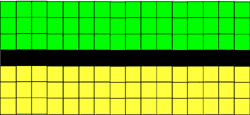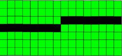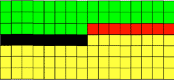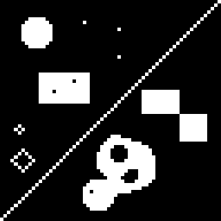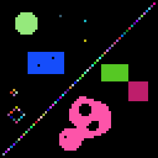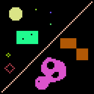Binary image 64×64 (zoom by a factor of 5)	86 foreground 4-connected regions	10 foreground 8-connected regions
(http://www.dca.fee.unicamp.br/projects/khoros/mmach/tutor/toolbox/basicl/labeling/front-page.html)

Region similarity

The uniformity or non-uniformity of pixels to form a connected region is represented by a uniformity predicate, i.e. a logical statement, or condition being true if pixels in the regions are similar with respect to some property (colour, grey level, edge strength, etc). A common predicate restricts signal variations over a neighbourhood: the predicate P(R), where R denotes a connected region, is TRUE if |f(x,y) − f(x+ξ,y+η)| ≤ Δ and FALSE otherwise (here, (x,y) and (x+ξ,y+η) are the coordinates of neighbouring pixels in region R. This predicate does not restrict the grey level variation within a region because small changes in signal values can accumulate over the region.
Intra-region signal variations can be restricted with a similar predicate: P(R) = TRUE if |f(x,y) − &mu_R| ≤ &Delta and FALSE otherwise where (x,y) is a pixel from the region R and μ_R is the mean value of signals f(x,y) over the entire region R.

Region growing

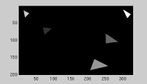
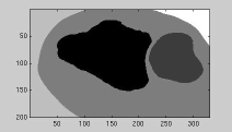
The bottom-up region growing algorithm starts from a set of seed pixels defined by the user and sequentially adds a pixel to a region provided that the pixel has not been assigned to any other region, is a neighbour of that region, and its addition preserves uniformity of the growing region.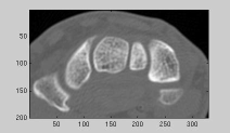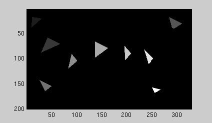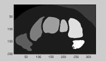

Greyscale image	Seed regions	Region growing results
(http://www.lems.brown.edu/~msj/cs292/assign5/segment.html)

Such a segmentation is simple but unstable. It is very sensitive to a chosen uniformity predicate, i.e. small changes of the uniformity threshold may result in large changes of the regions found. Also, very different segmentation maps are obtained under different routes of scanning an image, different modes of exhausting neighbours of each region, different seeds, and different types of pixel connectivity.

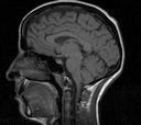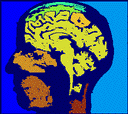Greyscale image (zoom by a factor of 2)	4-connected region growing	8-connected region growing
(http://www.comp.leeds.ac.uk/ai21/examples/images/rgrow.html)
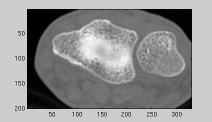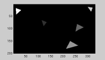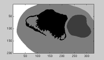Greyscale image	Seed regions: variant 1	Region growing results
	Seed regions: variant 2	Region growing results
(http://www.lems.brown.edu/~msj/cs292/assign5/segment.html)

Generally, a "good" complete segmentation must satisfy the following criteria:

1. All pixels have to be assigned to regions.
2. Each pixel has to belong to a single region only.
3. Each region is a connected set of pixels.
4. Each region has to be uniform with respect to a given predicate.
5. Any merged pair of adjacent regions has to be non-uniform.

Region growing satisfies the 3^rd and 4^th criteria, but not the others. The first two criteria are not satisfied because, in general, the number of seeds may not be sufficient to create a region for every pixel. The 5^th criterion may not hold because the regions grown from two nearby seeds are always regarded as distinct, even if those seeds are defined within a potentially uniform part of the image.

Split-and-merge segmentation

The top-down split-and-merge algorithm considers initially the entire image to be a single region and then iteratively splits each region into subregions or merges adjacent regions until all regions become uniform or until the desired number of regions have been established.
A common splitting strategy for a square image is to divide it recursively into smaller and smaller quadrants until, for any region R, the uniformity predicate P(R) is TRUE. The strategy builds a top-down quadtree: if P(image) is FALSE, the image is divided into four quadrants; if P(quadrant) is FALSE, the quadrant is divided into subquadrants; and so on:

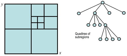
The splitting stage alternates with a merging stage, in which two adjacent regions R_i and R_j are combined into a new, larger region if the uniformity predicate for the union of these two regions, P(R_i ∪ R_j), is TRUE.

Texture segmentation: Spectral features

Grey level or colour pixel values by themselves are not sufficient for segmenting natural highly-textured images like those shown below: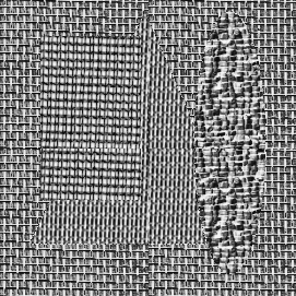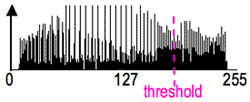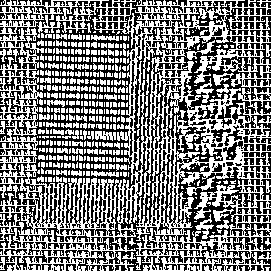

Textured collage	Grey-level histogram	Segmentation by thresholding

The above two regions (a black object and white background) obtained by simple thresholding are completely meaningless. To find meaningful regions containing different types of homogeneous textures, specific texture measures (features) have to be used like, for example, local spatial signal statistics:

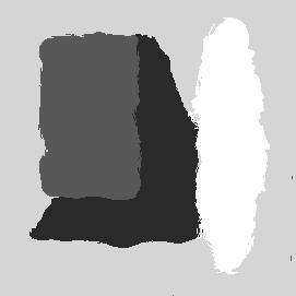Textured collage	Segmentation using local features
(http://www.sztaki.hu/~sziranyi/textu-iu.html)
Textured collage, actual region map, and segmentation using local features
(http://www.ercim.org/publication/Ercim_News/enw64/mikes.html

Texture is a spatial property that characterises groups of pixels. A local measure of texture is therefore computed over a neighbourhood. An example of the simplest statistical measure is the variance of grey levels in a square n×n neighbourhood centred on a pixel:

The "variance" image presents scaled standard deviations σ for each pixel; bright regions in this image signify high local variance of grey levels:

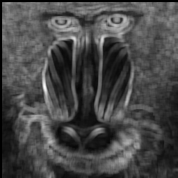Greyscale image "Baboon"	Variance image (7×7 window)
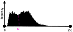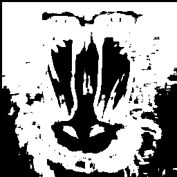Histogram of the variance image	Variance thresholding: T=63

For most of natural textures, simple statistical measures are of little use. If two textures of interest are periodic, they might be separated in the frequency domain by comparing the spectra of small samples taken from the two patterns. Spectral segmentation techniques typically use the radially or angularly integrated power spectrum of a region in an image. Radial integration sums power values within a ring of radius r and width Δr. Angular integration sums power values within a sector defined by a radius, r, an orientation, θ, and an angular width, Δθ. The ring-based measurement relates to the texture scale: a concentration of power at small or large radii signifies coarse or fine texture, respectively. The sector-based measurement relates to texture orientation: a texture oriented in a direction φ results in high power for a sector at angle θ = φ + π/2.

References

These lecture notes follow Chapter 10 "Segmentation" of the textbook

• Nick Efford. Digital Image Processing: A Practical Introduction Using Java^TM. Pearson Education, 2000.

with extra examples and teaching materials taken mostly, with corresponding references, from the Web.
Return to the local table of contents
Return to the general table of contents